Checking sequence of instructions
In order to keep track of which line of the program is currently being executed, a new registry called “program counter” is added to the state machine. We denote it by because it is verified in a zero-knowledge manner. The is therefore a new column of the execution trace and it contains, at each clock, the line in the zkASM program of the instruction being executed.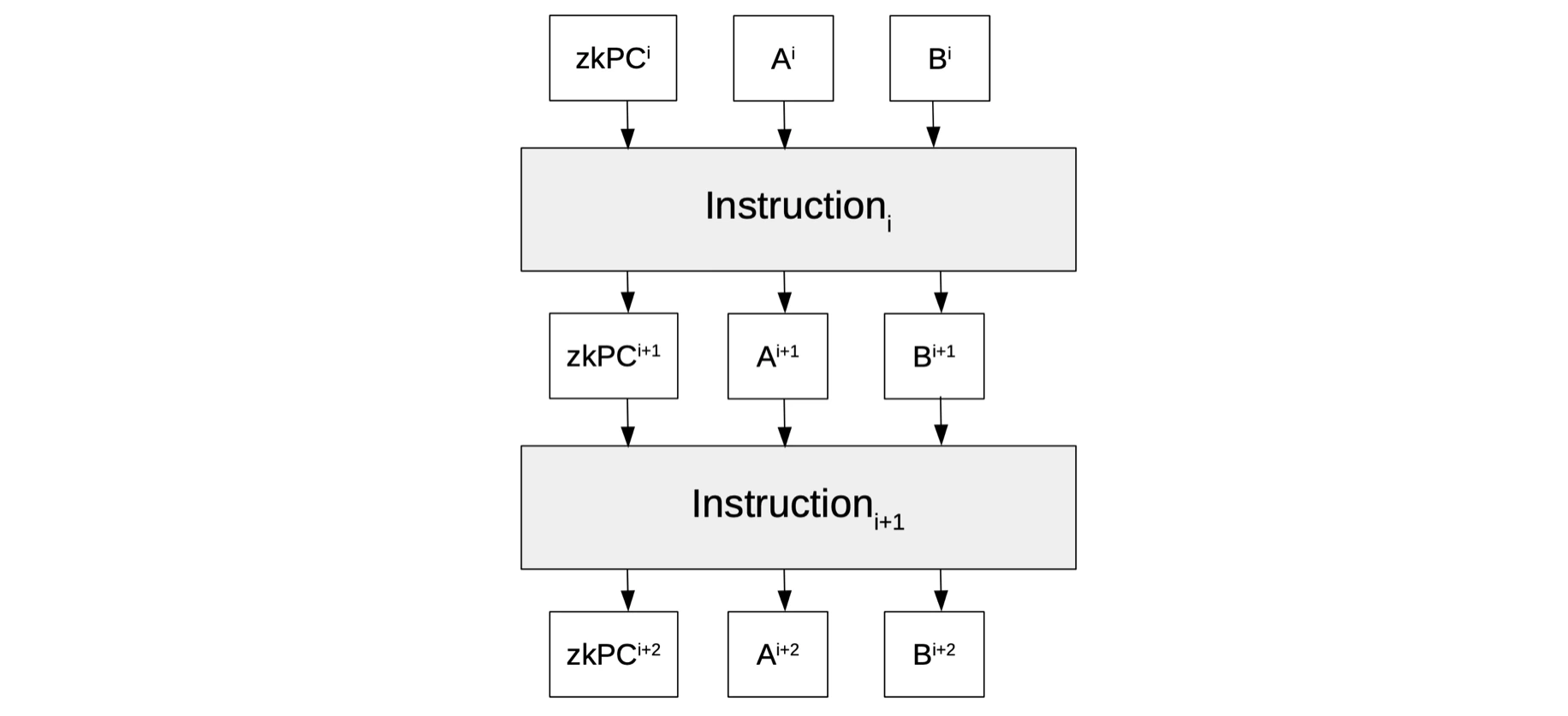
Program counter constraint related to JMP
This is how the instruction is implemented: A new selector called is added, as a column to the execution trace. And, the program counter now uses the following identity to keep track of the correct line of the assembly program to be executed next; therefore acts as a ‘flag’ where;- , if is not activated (i.e., if is ), or
- , if is activated (i.e., if is ).
Program counter constraint related to JMPZ
The similarly needs a selector to be added as an extra column to the execution trace, call it . Since the instruction is executed only on condition that is zero, we introduce a flag called , such that; if , and if . This means and satisfy the following constraint, Note that is a field element, and every non-zero element of the prime field has an inverse. That is, exists if and only if . The following constraint together with can be tested to check whether and are as required, Since only if is the very instruction in the line currently being executed, and only if . It follows that the factor only if both and hold true. Hence, the following constraint enforces the correct sequence of instructions when is executed; In order to ascertain correct execution of the instruction, it suffices to check the above three constraints; , and . Note that is not part of any instruction. The evaluations of therefore have to be included in the execution trace as a committed polynomial, and thus enables checking the first identity, . Most importantly, we rename the polynomial as .Program counter constraint related to JMP and JMPZ
All four constraints, , , and can be merged as follows; Define "" as an intermediate polynomial, where is provided as part of the jump instructions, and . We now have the following new columns in the execution trace: With the intermediate definition in , we are preparing the path to expanding the definition, for example, to include other sources (apart from instructions) from which to get the destination address in jumps.Correct program ending with a loop
We have previously resorted to ending our program by repeating the "" instruction. This was not the best solution. To properly finish our programs, we need to ensure that the execution trace generated from the assembly is cyclic. We therefore utilise a loop while the current is less than , a step before the last step of the execution trace. That is, before jumping back to the start, with the instruction, the current is checked with the function "". So, we query the executor for when the execution trace is at its last but one row, with the following line of code,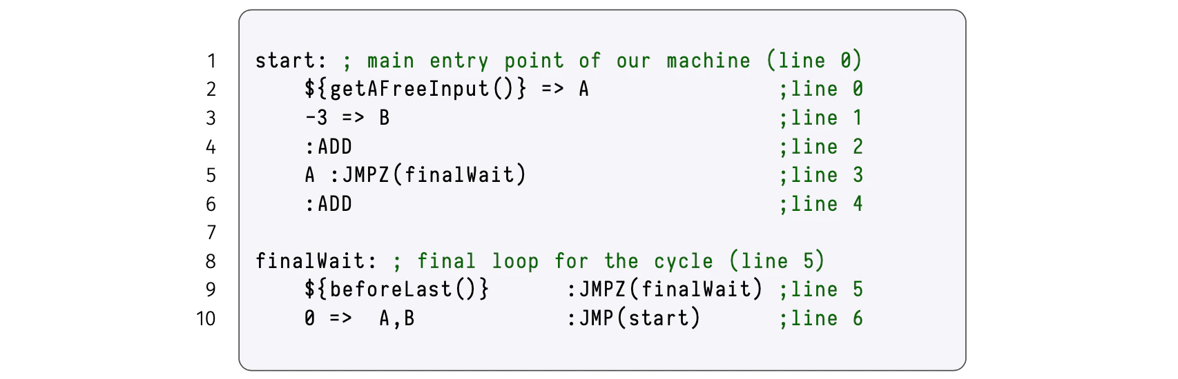
Commentary on the execution trace
The intention here to give a step-by-step commentary on the execution trace for the Assembly code in Figure 8 above, for a free input equal to and a trace size (interpolation size) equal to . We show the values corresponding to each of the execution trace, particularly for,- The committed polynomials that form part of the instruction; , , , , , , , , , and .
- The committed polynomials that are only part of the trace; , , , , and .
- The intermediate polynomials , which are just intermediate definitions; , and .