Intermediate steps

The first step of the proof recursion, where the first STARK proof is verified, is referred to as recursive1. All intermediate steps of recursion are referred to as recursive2, while the last step is called recursivef.

Setup S2C for recursive1

At this point, the first STARK proof \(\pi\) has been validated with a STARK proof \(\pi_\texttt{c12a}\).

The idea now is to generate a CIRCOM circuit that verifies \(\pi_\texttt{c12a}\), by mimicking the FRI verification procedure.

In order to achieve this, a verifier circuit c12a.verifier.circom is generated from the previously obtained files;

• the c12a.pil file,
• the c12a.starkinfo parameters, and
• the constant root c12a.verkey.constRoot,

by filling the \(\mathtt{stark\_} \texttt{verifier.circom.ejs}\) template as before.

In this case, as mentioned in the Normalization stage subsection of the Recursion section, in order to include the constant root as a public input, the circuit had to be slightly modified.

This will be extremely important in the Aggregation stage, where all the constants for the computation, which depend on the previous circuit, need to be provided as public inputs.

This is done by using the recursive1.circom file and importing inside the previously generated c12a.verifier.circom circuit as a library.

The verifier circuit is instantiated inside \(\mathtt{recursive1.circom}\), connecting all the necessary wires and including the constant root to the set of publics.

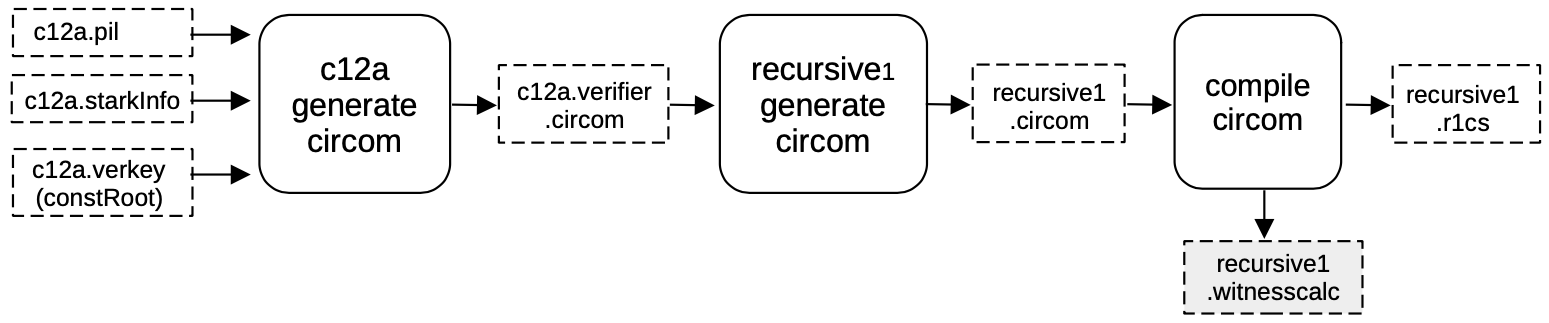
The output circom file recursive1.circom , is compiled into a R1CS recursive1.r1cs file and a witness calculator program, \(\mathtt{recursive1.witnesscal}\), which will be used for both building and filling the next execution trace.

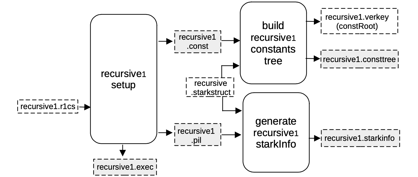
Setup C2S for recursive1

As seen previously, a machine-like construction, whose correct execution is equivalent to the validity of the previous circuit, is obtained from the R1CS description of the verification circuit.

In this case, the R1CS description is in the file recursive1.r1cs, and the obtained construction is described by recursive1.pil.

Again, a binary for all the constant polynomials recursive1.const is generated, together with the helper file recursive1.exec, which provides allocation of the witness values into their corresponding positions in the execution trace.

Note that all the FRI-related parameters are stored in a recursive.starkstruct file (located in the prover repository), and it is coupled with,

• the recursive1.pil file as inputs to the \(\mathtt{generate\_starkinfo}\) service in order to generate the recursive1.starkinfo file, and
• the recursive1.const as inputs to the component that builds the Merkle tree of evaluations of constant polynomials, recursive1.consttree, and its root recursive1.verkey.

In this case, a blowup factor of \(2^4 = 16\) is used, and thus allowing the number of queries to be \(32\).

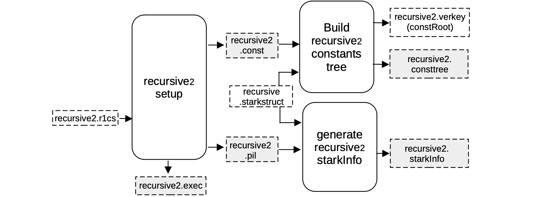
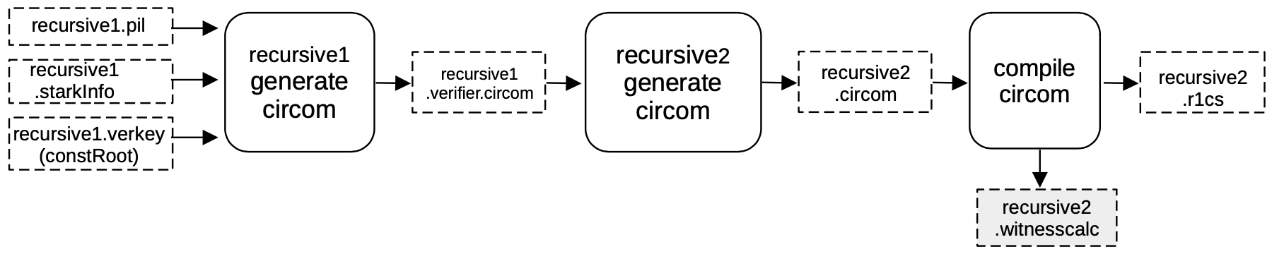
Setup S2C for recursive2

As before, a CIRCOM circuit is generated that verifies \(\mathtt{π_{rec1}}\) by imitating the FRI verification procedure.

In order to do this, a verifier circuit recursive1.verifier.circom is generated from the previously obtained files;

• the recursive1.pil file,
• the recursive1.starkinfo file, and
• the constant root recursive1.verkey.constRoot,

by filling the verifier \(\mathtt{stark\_verifier.} \texttt{circom.ejs}\) template.

Once the verifier is generated using the template, the template is used to create another CIRCOM that aggregates two verifiers.

Note that, in the previous step, the constant root was passed hardcoded from an external file into the circuit.

That’s the very reason for having the Normalization stage: enabling the previous circuit and anyone verifying each or both proofs to have the exact same form, and thus allowing iterated recursion.

Henceforth, the recursive2.circom circuit has two verifiers and two multiplexors that are actually deciding the form of each of the verifiers:

• if the proof is \(\mathtt{\pi_{rec1}}\)-type, the hardcoded constant root is input, but
• if the proof is a \(\mathtt{\pi_{rec2}}\)-type, the constant root should be connected as an input signal, coming from a previous circuit.

A schema of the recursive2 circuit generated is as shown in the below Figure.

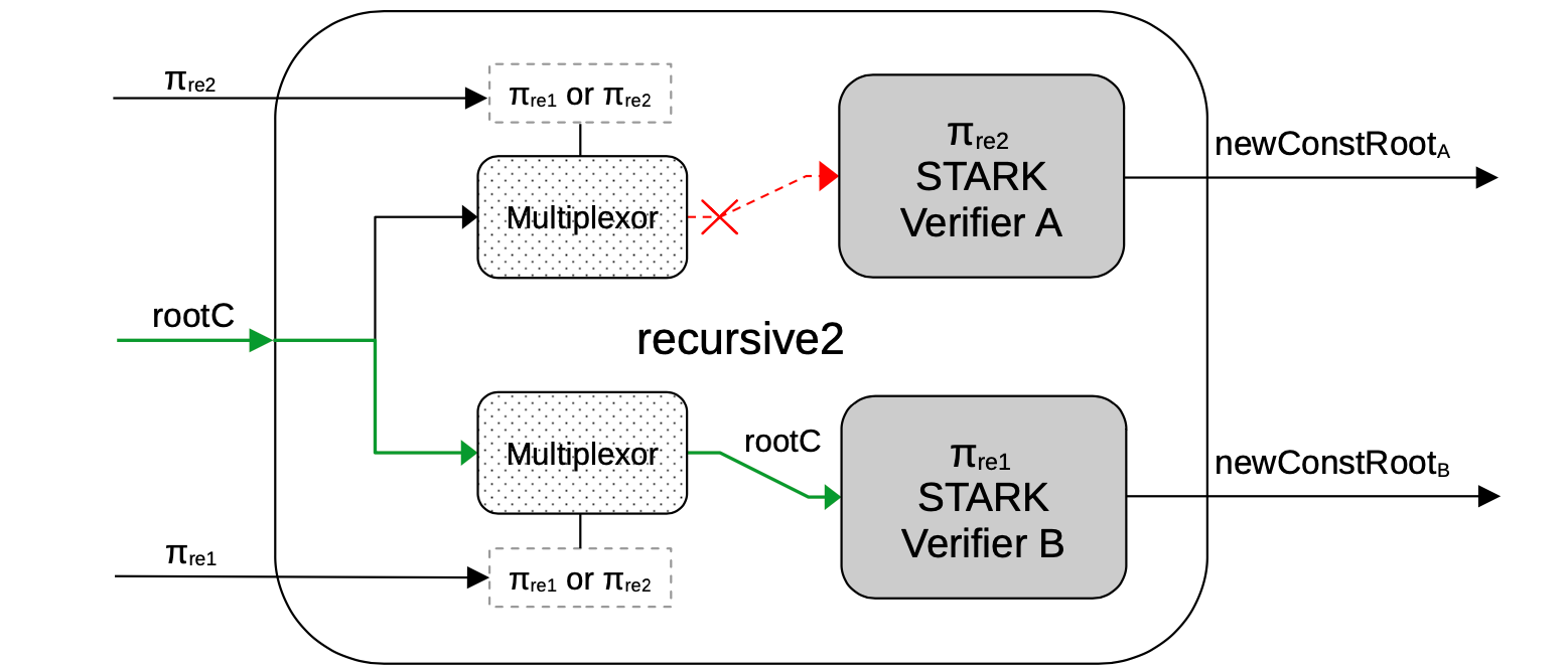
Observe that, since the upper proof is of the \(\mathtt{\pi_{rec2}}\)-type, the Multiplexor does not provides the constant root rootC to the Verifier A for hardcoding it, because this verifier should get it through a public input from the previous circuit.

Otherwise, since the lower proof has the \(\mathtt{\pi_{rec1}}\)-type, the Multiplexor lets it pass through by providing the constant root to the Verifier B, so that it can be hardcoded when the corresponding template is filled.

The output CIRCOM file recursive2.circom , is obtained by running a different script called genrecursive which is compiled into an R1CS recursive2.r1cs file and a witness calculator program recursive2.witnesscal and they will both be used, later on, to build and fill the next execution trace.

Setup C2S for recursive2

As seen before, when executing a C2S, a machine-like construction gets obtained from the R1CS description of the verification circuit.

This construction is specifically the one whose execution correctness is equivalent to the validity of the previous circuit. And it is described by a PIL recursive2.pil file.

The R1CS description taken as input to produce this construction is in the file recursive2.r1cs.

The other outputs of the recursive2 setup component are;

• A binary for all the constant polynomials recursive2.const, and
• The helper file recursive2.exec, which provides allocation of the witness values into their corresponding positions in the execution trace.

Note that all the FRI-related parameters are stored in a recursive.starkstruct file, and in the next step, it is paired up with,

• the recursive1.const as inputs to the component that builds the Merkle tree of evaluations of constant polynomials, recursive2.consttree and its root recursive2.verkey.
• the recursive2.pil file as inputs to the \(\mathtt{generate\_starkinfo}\) service in order to generate the recursive1.starkinfo file.

In this case, we are using the same blowup factor of \(2^4 = 16\), allowing the number of queries to be \(32\).