Merkle trees
zkProver’s data is stored in the form of a special Sparse Merkle Tree (SMT), which is a tree that combines the concept of a Merkle Tree and that of a Patricia tree. The design is based on how the Sparse Merkle Trees are constructed and how they store keys and values.
Tip
The content of this document is rather elementary. Experienced developers can fast-forward to later sections and only refer back as the need arises.
A typical Merkle tree has leaves, branches and a root. A leaf is a node with no child-nodes, while a branch is a node with child-nodes. The root is therefore the node with no parent-node.
See the below figure for an example of how a hash function \(\mathbf{H}\) is used to create a Merkle tree recording eight values;
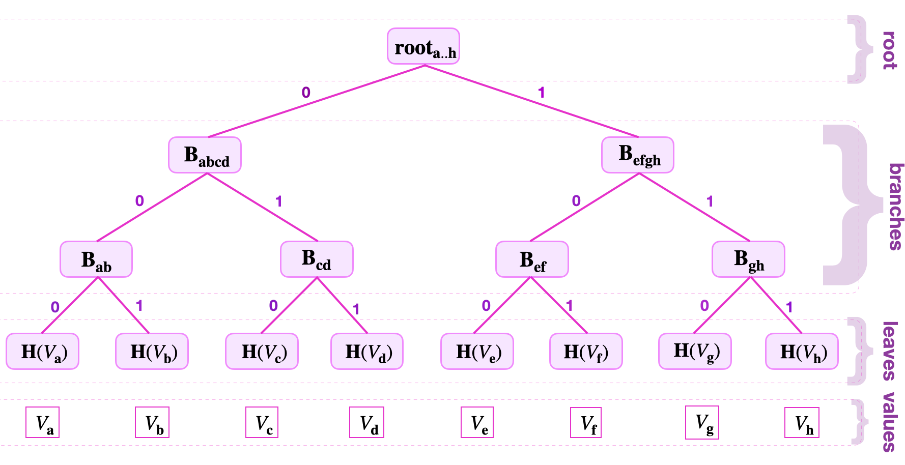
Firstly, each leaf is nothing but the hash value \(\mathbf{H}(\text{V}_{\mathbf{i}})\) of a particular value \(\text{V}_{\mathbf{i}}\), where \(\mathbf{i}\) is an element of the index-set \(\{ \mathbf{a}, \mathbf{b}, \mathbf{c}, \mathbf{d}, \mathbf{e}, \mathbf{f}, \mathbf{g}, \mathbf{h} \}\).
Secondly, the branch nodes are computed as follows;
Thirdly, the root is computed as \(\mathbf{root}_{\mathbf{a..h}} = \mathbf{H} \big(\mathbf{B}_{\mathbf{abcd}}\| \mathbf{B}_{\mathbf{efgh}} \big)\).
Leaves that share a parent-node are called siblings. The same terminology applies to branches. For example, \(\mathbf{B}_{\mathbf{ab}}\) and \(\mathbf{B}_{\mathbf{cd}}\) are sibling branches because they are branches of the same parent, \(\mathbf{B}_{\mathbf{abcd}}\). Similarly, \(\mathbf{B}_{\mathbf{efgh}}\) and \(\mathbf{B}_{\mathbf{abcd}}\) are sibling branches.
Keys and navigating a Merkle tree
Note the bits used to label edges in figure above. The strings of these bits are called Keys, and they indicated where a node is located in a Merkle Tree. Since these keys uniquely locate nodes, they are used to navigate from the root to the leaves (and backwards).
Suppose one is given the key-value pair \(( K_{\mathbf{d}} , V_{\mathbf{d}})\), where the key is \(K_{\mathbf{d}} = 10010110\).
In order to locate the key-value pair \(( K_{\mathbf{d}} , V_{\mathbf{d}})\) in the Merkle depicted in the figure above, the key \(K_{\mathbf{d}}\) is read bit-by-bit from the right-most bit to the left-most bit. While traversing the tree from the root downwards,
-
a zero-key-bit “\(0\)” means “follow the edge going to the left”,
-
a key-bit “\(1\)” means “follow the edge going to the right”.
Since \(K_{\mathbf{d} } = 10010110\), as follows:
- Read the least-significant bit of \(K_{\mathbf{d}}\), which is \(0\), hence traverse the tree to the left, and reach \(\mathbf{B_{abcd}}\).
- Then read the second significant key-bit, which is “\(1\)” in this case. So take the edge going to the right, reaching \(\mathbf{B_{cd}}\).
- Again, read the next key-bit, which is “\(1\)”, hence follow the edge going to the right, reaching the leaf \(\mathbf{H}( V_{\mathbf{d}} )\).
Since \(\mathbf{H}( V_{\mathbf{d}})\) is a leaf and not a branch, and the navigation was correctly done with respect to the given key \(K_{\mathbf{d}}\), the \(\mathbf{H}( V_{\mathbf{d}})\) must be the leaf storing the value \(V_{\mathbf{d}}\).
One can similarly climb the tree, going in the reverse direction, by using the key-bits of the given key in the reverse order. That is, starting with the last key-bit used to reach the leaf and ending with the least-significant bit of the key.
The tree-address of the value \(V_{\mathbf{x}}\), herein refers to the position of the leaf \(L_{\mathbf{x}} := \mathbf{H}( V_{\mathbf{x}})\), denoted by the key-bits used to reach \(L_{\mathbf{d}}\) but in the reverse order.
In the above example, the tree-address of \(V_{\mathbf{d}}\) is 011.
A Merkle proof example
Merkle Trees can be used as commitment schemes. And here is an example that follows the (key,value)-pair approach used in the zkProver. Consider the Merkle Tree shown in the figure above.
If the prover has committed to a value \(\text{V}_{\mathbf{f}}\) by appending a new leaf \(\mathbf{H}(\text{V}_{\mathbf{f}})\) to the Merkle Tree as depicted in the above figure, he must then avail the following information, to enable verification of his claim;
- The Merkle root, denoted by \(\mathbf{root}_{\mathbf{a..h}}\),
- The value \(\text{V}_{\mathbf{f}}\), and
- The siblings; \(\mathbf{H}(\text{V}_{\mathbf{e}})\), \(\mathbf{B}_{\mathbf{gh}}\) and \(\mathbf{B}_{\mathbf{abcd}}\).
Instead of searching through all hash values stored in the tree, the verifier uses only a few hash values of relevant siblings. That is, three siblings in this case.
The verifier then checks the prover’s claim by computing the Merkle root as follows;
-
He computes \(\mathbf{H}(\text{V}_{\mathbf{f}})\), which is the hash of the value \(\text{V}_{\mathbf{f}}\).
-
Then uses the sibling \(\mathbf{H}(\text{V}_{\mathbf{e}})\) to compute \(\mathbf{H} \big( \mathbf{H}(\text{V}_{\mathbf{e}})\|\mathbf{H}(\text{V}_{\mathbf{f}}) \big) =: \tilde{ \mathbf{B}}_{\mathbf{ef}}\), which should be the same as the branch node \(\mathbf{B}_{\mathbf{ef}}\).
-
Next, he computes \(\mathbf{H} \big( \tilde{ \mathbf{B}}_{\mathbf{ef}}\|\mathbf{B}_{\mathbf{gh}} \big) =: \tilde{ \mathbf{B}}_{\mathbf{efgh}}\), corresponding to the branch node \(\mathbf{B}_{\mathbf{efgh}}\).
-
Now, uses \(\mathbf{H} \big( \mathbf{B}_{\mathbf{abcd}}\| \tilde{ \mathbf{B}}_{\mathbf{efgh}} \big) =: \tilde{ \mathbf{root}}_{\mathbf{a..h}}\).
The Merkle proof is concluded by checking whether \(\tilde{ \mathbf{root}}_{\mathbf{a\dots h}}\) equals to the publicly known root \(\mathbf{root}_{\mathbf{a..h}}\).
Note
The symbol tilde denoted \(\tilde{\Box}\), is used throughout the document to indicate
that the computed value, \(\tilde{\Box}\), still needs to be checked, or tested to be true.