Implementing EGP strategy
In this section we provide an elaborate discussion on how Polygon zkEVM network ensures transactions are executed with the best gas price for the user, while incurring minimal or no losses.
You will learn how to sign transactions with the appropriate gas price ensuring:
- There is minimal likelihood for your transactions to be reverted.
- The sequencer prioritizes your transactions for execution.
How to avert rejection of transactions
The first step is to ensure that users sign transactions with sufficient gas price, and thus ensure the transactions are included in the L2’s pool of transactions.
Polygon zkEVM’s strategy is to use pre-execution of transactions so as to estimate each transaction’s possible gas costs.
Suggested gas prices
Due to fluctuations in the L1 gas price, the L2 network polls for L1 gas price every 5 seconds.
The polled L1 gas prices are used to determine the appropriate L2 gas price to suggest to users.
Since the L1 gas price is likely to change between when a user signs a transaction and when the transaction is pre-executed, the following parameters are put in place:
- A \(5\)-minute interval of several suggested gas prices, called \(\texttt{MinAllowedPriceInterval}\).
- During the \(\texttt{MinAllowedPriceInterval}\), the user’s transactions can be accepted for pre-execution, provided the \(\texttt{SignedGasPrice}\) is higher than the lowest suggested gas price in the interval.
- The lowest among the suggested gas prices is called \(\texttt{L2MinGasPrice}\).
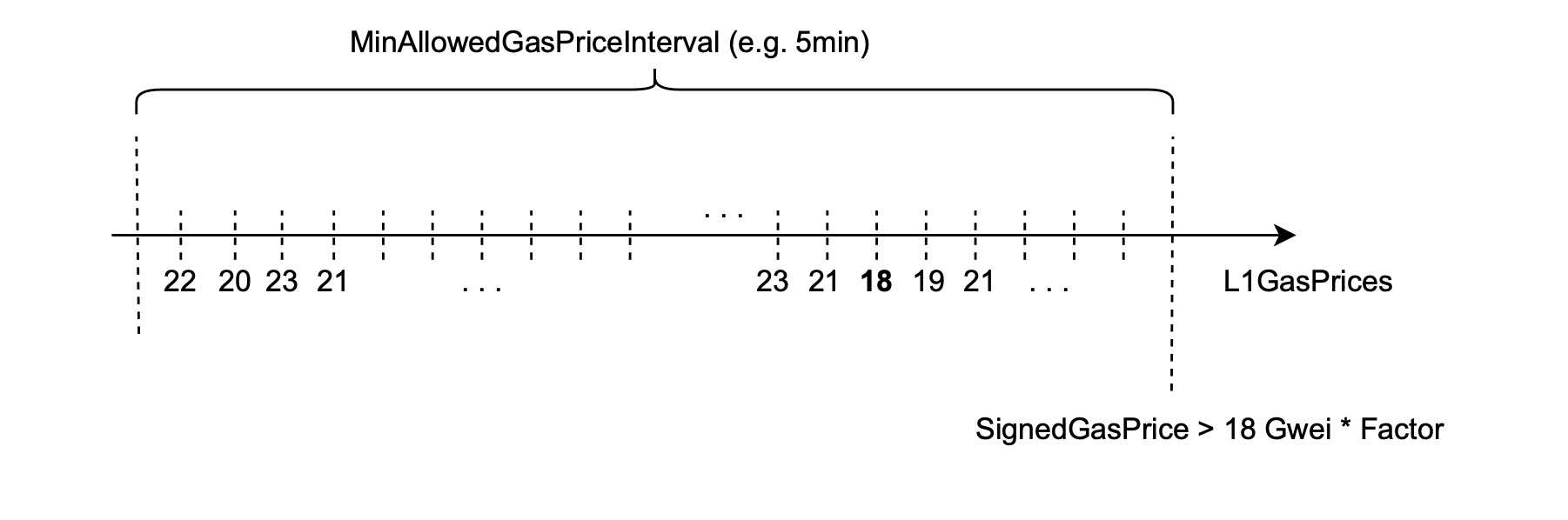
All transactions such that \(\texttt{SignedGasPrice} > \texttt{L2MinGasPrice}\) are accepted for pre-execution.
How to avoid incurring losses in L2
There are three measures put in place to help avoid incurring gas price-induced losses in the L2 network:
- Pre-execution of transactions.
- The breakeven gas price: \(\texttt{BreakEvenGasPrice}\).
- The L2’s net profit.
Transaction pre-execution
You can use pre-execution to estimate the L2 resources each transaction will spend when processed.
These resources are measured in terms of counters in the zkEVM’s ROM, but are converted to gas units for better UX.
This is the stage where transactions are either discarded or stored in the pool database, a pool of transactions waiting to be processed by the sequencer.
The price of posting transaction data to L1 is charged to the zkEVM network at a full L1 price.
Although computational costs in L2 may be accurately estimated, in cases where there is a reduction in such costs due to fewer L2 resources being spent, the user may be justified to sign a transaction with a very low gas price. But by signing such a low gas price, the user runs the risk of exhausting their wei reserves when transaction data is posted to L1.
So then, if the use of \(\texttt{L1GasPriceFactor = 0.04}\) is the only precautionary measure the L2 network takes in computing suggested gas prices, the L2 network will most likely incur losses.
A \(\texttt{suggestedFactor = 0.15}\) is therefore used to calculate each suggested gas price:
The need for such a factor originates from the fact that the sequencer is obliged to process every transaction stored in the pool database, irrespective of its \(\texttt{SignedGasPrice}\) and the prevailing L1 gas price.
Breakeven gas price
Calculating the breakeven gas price is another measure used in the Polygon zkEVM network to mitigate possible losses.
As explained before, the computation is split in two; costs associated with data availability, and costs associated with the use of resources when transactions are processed.
Costs associated with data availability
The cost associated with data availability is computed as,
where \(\texttt{DataCost}\) is the cost in gas for data stored in L1.
The cost of data in Ethereum varies according to whether it involves zero bytes or non-zero bytes. In particular, non-zero bytes cost \(16\) gas units, while zero bytes cost \(4\) gas units.
Also, recall that the computation of the cost for non-zero bytes must take into account constants that appear in transactions but are not included in the RLP, which includes:
- The signature, which consists of \(65\) bytes.
- The previously defined \(\texttt{EffectivePercentageByte}\), which consists of a single byte.
This results in a total of \(66\) constantly present bytes.
Taking everything into consideration, \(\texttt{DataCost}\) can be computed as:
where \(\texttt{TxNonZeroBytes}\) represents the count of non-zero bytes in a raw transaction, and similarly \(\texttt{TxZeroBytes}\) represents the count of zero bytes in a raw transaction sent by the user.
Computational costs
Costs associated with transaction execution is denoted by \(\texttt{ExecutionCost}\), and is measured in gas.
In contrast to costs for data availability, calculating computational costs requires executing transactions.
So then,
The total fees received by L2 are calculated with the following formula:
where \(\texttt{L2GasPrice}\) is obtained by multiplying \(\texttt{L1GasPrice}\) by a chosen factor less than \(1\),
In particular, we choose a factor of \(0.04\).
Total price of a transaction
The total transaction cost is simply the sum of data availability and computational costs:
In order to establish the gas price at which the total transaction cost is covered, we can compute \(\texttt{BreakEvenGasPrice}\) as the following ratio:
Additionally, we incorporate a factor \(\texttt{NetProfit ≥ 1}\) that allows us to achieve a slight profit margin:
We then conclude that it is financially safe to accept the transaction if
However, a problem arises:
In the RPC component, we’re only pre-executing the transaction, meaning we’re using an incorrect state root. Consequently, the \(\texttt{GasUsed}\) is only an approximation.
This implies that we need to multiply the result by a chosen factor before comparing it to the signed price to hedge against unforeseen costs.
This ensures that the costs are covered in case more gas is ultimately required to execute the transaction. This factor is named \(\texttt{BreakEvenFactor}\).
Now we can conclude that if
then it is safe to accept the transaction.
Observe that we still need to introduce gas price prioritization, which we explain later.
Example (Breakeven gas price)
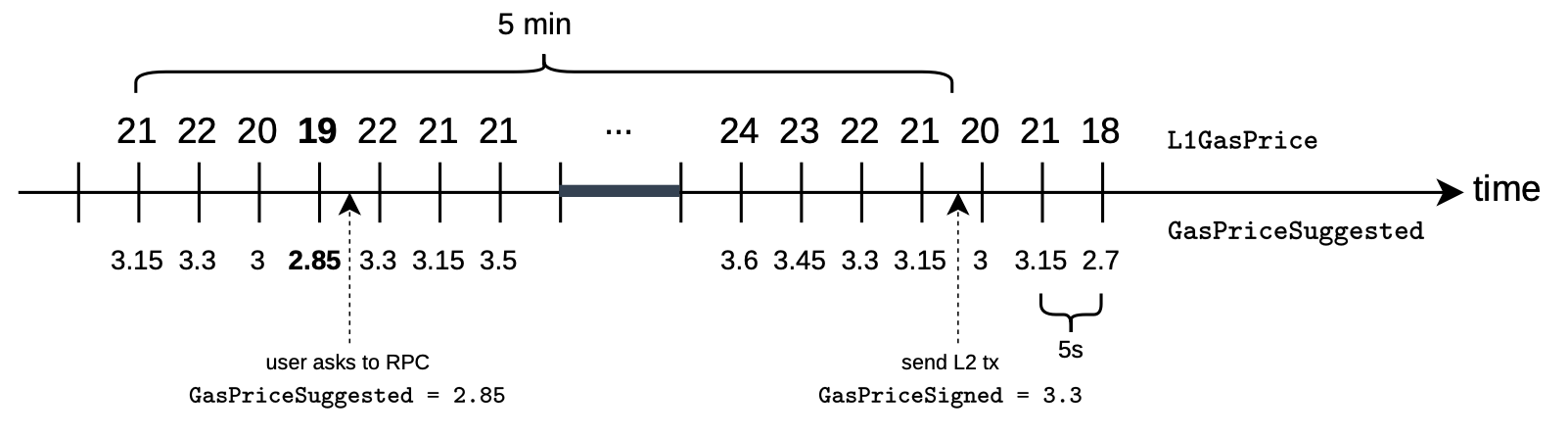
Recall the example proposed before, where the \(\texttt{GasPriceSuggested}\) provided by RPC was \(2.85\) gwei per gas, but the user ended up setting \(\texttt{SignedGasPrice}\) to \(3.3\).
The figure below depicts the current situation.
Suppose the user sends a transaction that has \(200\) non-zero bytes, including the constants and \(100\) zero bytes.
Moreover, on pre-executing the transaction without an out-of-counters (OOC) error, \(60,000\) gas units are consumed.
Recall that, since we are using a “wrong” state root, this amount is only an estimation.
Hence, using the previously explained formulas, the total transaction cost is:
Observe that the \(21\) appearing in the substitution is the \(\texttt{L1GasPrice}\) at the time of sending the transaction.
Now, we are able to compute the \(\texttt{BreakEvenGasPrice}\) as:
We have introduced a \(\texttt{NetProfit}\) value of \(1.2\), indicating a target of a \(20\%\) gain in this process.
At first glance, we might conclude the transaction has been accepted:
but, recall that this is only an estimation, the gas consumed with the correct state root can differ.
To avoid this, we introduce a \(\texttt{BreakEvenFactor}\) of \(30\%\) to account for estimation uncertainties:
Consequently, the system accepts the transaction.
Example (Breakeven factor)
Suppose we disable the \(\texttt{BreakEvenFactor}\) by setting it to \(1\).
Our original transaction’s pre-execution consumed \(60,000\) gas:
However, let’s assume the correct execution at the time of sequencing consumes \(35,000\) gas.
If we recompute \(\texttt{BreakEvenGasPrice}\) using this updated used gas, we get \(3.6\ \texttt{GWei/Gas}\), which is way higher than the original estimation.
That means we should have charged the user a higher gas price in order to cover the whole transaction cost, standing at \(105,000\ \texttt{GWei}\).
But, since we are accepting all the transactions that sign more than \(2.85\) of gas price, we do not have any margin to increase it.
In the worst case we are losing:
By introducing \(\texttt{BreakEvenFactor}\), we are limiting the accepted transactions to the ones with,
in order to compensate for such losses.
In this case, we have the flexibility to avoid losses and adjust both the user’s and Polygon zkEVM network’s benefits since:
Final Note: In the above example, even though we assume that a decrease in the \(\texttt{BreakEvenGasPrice}\) is a result of executing with a correct state root, it can also decrease significantly due to a substantial reduction in \(\texttt{L1GasPrice}\).