Introduction

The zkEVM prover is a software component with which the zkEVM generates proofs that attest to correct execution of programs given a specific set of inputs.

While the process of generating a proof is resource-intensive, the time required to verify the proof is significantly shorter, enabling verification to be carried out by a smart contract.

On a high level, the prover takes the last batch and the current state as inputs in order to calculate the new state, together with a proof that attests to the computational integrity of the state transition.

The figure below depicts a typical state transition \(\big(S_{i}^{L2_x} \to S_{i+1}^{L2_x}\big)\),

• Taking as inputs, a batch \(\mathtt{Batch}_i\) and the current L2 state \(S_{i}^{L2_x}\).
• And the output as a new L2 state \(S_{i+1}^{L2_x}\), together with a proof \(\pi_{i+1}\).

The initial step to produce a proof involves creation of an execution matrix, which is a matrix that records all intermediate computations constituting a larger computation. Such a matrix is also called an execution trace.

This larger computation can be thought of as the state transition function, while the smaller intermediate computations are like the zkEVM instructions or opcodes.

As we will later on see, it may take one or more zkEVM opcodes to implement a single EVM opcode.

This indicates the lack of a strict one-to-one correspondence between EVM opcodes and the Polygon zkEVM’s.

Typical execution matrix

Unless otherwise stated, we use a matrix with three columns; \(\texttt{A}\), \(\texttt{B}\) and \(\texttt{C}\).

Furthermore, suppose the number of rows is bounded by some constant \(N\), which we will call length of the execution trace.

The columns of an execution trace are often called registers. So, the terms “column” and “register” are used interchangeably in this document.

We depict an execution trace of length \(N\), having three registers \(\texttt{A}\), \(\texttt{B}\) and \(\texttt{C}\), in the figure below.

\[ \begin{aligned} \begin{array}{|c|c|c|c|c|}\hline \bf{\texttt{ A }} & \bf{\texttt{ B }} & \bf{\texttt{ C }}\\ \hline a_0 & b_0 & c_0 \\ \hline a_1 & b_1 & c_1 \\ \hline \dots & \dots & \dots \\ \hline a_N & b_N & c_N \\ \hline \end{array} \end{aligned} \]

A toy example (Execution matrix)

Suppose we are given a set of three input values, \(x := (x_0, x_1, x_2)\), and we want to use an execution trace to model the following computation:

\[ [(x_0 +x_1)·4]·x_2 \]

Let us also suppose that the only available instructions (or operations) are those described below:

1. Copy inputs into cells of the execution trace.

2. \(\texttt{ADD}\) instruction: Add two values in cells on the same row, and leave the result in the first cell of the next row.

3. \(\texttt{TIMES4}\) instruction: Multiply a given value by a constant, and leave the result in the first cell of the next row.

4. \(\texttt{MUL}\) instruction: Multiply two values in cells on the same row, and leave the result in the first cell of the next row.

Let’s provide a specific example by setting the input \(x\) to \(x := (1, 2, 5)\).

Substituting the input values in the given computation yields:

\[ [(x0 +x1)·4]·x2 =[(1+2)·4]·5=60 \]

The corresponding execution trace, using only the above-mentioned operations, is as follows:

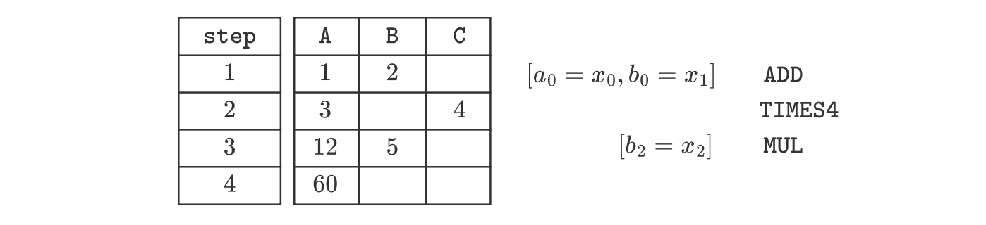
Let’s take a step-by-step walk-through the above execution trace:

1. First of all, we use the instruction that copies the inputs \(1\) and \(2\) into the columns \(\texttt{A}\) and \(\texttt{B}\), respectively. And then invoke the \(\texttt{ADD}\) instruction.
2. After executing the \(\texttt{ADD}\) instruction, the second row of register \(\texttt{A}\) now holds the sum of \(1\) and \(2\), that is the value \(3\). At this point we utilize the \(\texttt{TIMES4}\) instruction to obtain \(3 \cdot 4 = 12\), and place it in the first cell of row 3.
3. Now, with \(12\) in the third row of register \(\texttt{A}\), we proceed to copy the third input, \(5\), into register \(\texttt{B}\). Then the \(\texttt{MUL}\) instruction is invoked to multiply the current two values in row 3. (viz. \(12\) and \(5\)). The resulting outcome (which is \(60\)) of the \(\texttt{MUL}\) instruction is placed in the first cell of row 4.
4. Consequently, this last outcome \(60\) is in fact the final output for the entire computation.

Observe that we have only used the available instructions as proposed in our scenario.

Notice that for a specific computation, and except for the entries in the matrix, the shape of the execution matrix remains the same irrespective of the variable input values \(x = (x_0, x_1, x_2)\).

For example, if \(x = (5, 3, 2)\) for the same program, the resulting execution matrix is as follows:

However, if we examine the columns in the above execution trace, we can identify two distinct types of columns:

• Witness columns: Values in these columns depend on the input values. They change whenever different input values are used. In the above example, columns \(\texttt{A}\) and \(\texttt{B}\) are witness columns.
• Fixed columns: Values in these columns remain unaffected by changes in the input values. In the above example, column \(\texttt{C}\) is a fixed column, and it is only used to store the constant \(4\).

In each case of the above example, the constant \(4\) is used in the second step of the computation, when the \(\texttt{TIMES4}\) instruction is invoked.