Execution trace design

In this section we discuss some aspects pertaining to the shapes or dimensions of the execution traces.

The intention is to ensure that each row of an execution trace contains all data required to validate a single or part of a zkASM operation.

Notation

Since execution traces are created in the context of state machines, columns of a execution trace are also referred to as registries.

A registry \(\texttt{A}\) is denoted by \(\texttt{A} = ( a_0, a_1, ... , a_{2^{k}-1})\), where each \(a_{i+1}\) is the value in \(\texttt{A}\) subsequent to \(a_i\). Denote this next value in \(\texttt{A}\) by \(a'\). That is, \(a' = a_{i+1}\).

Each \(a'\) is typically the output of some operation \(\texttt{Op}\), applied on some entries \((a_{i}, b_{i}, c_{i})\) from columns \(\texttt{A}\), \(\texttt{B}\) and \(\texttt{C}\). That is:

\[ a' = \texttt{Op}\big( a_{i}, b_{i}, c_{i} \big) \]

Example: (Fitting all variables in few columns)

Consider the three operations, \(\texttt{Op1}\), \(\texttt{Op2}\) and \(\texttt{Op3}\), as instructions to the executor, written in zkASM.

These operations, \(\texttt{Op1}\), \(\texttt{Op2}\) and \(\texttt{Op3}\), are defined to change the next entry of the registry \(\texttt{A} = ( a_0, a_1, ... , a_{2^{k}-1})\) as follows:

\[ \begin{aligned} &\texttt{Op1}:a' =a+b+c\\ &\texttt{Op2}:a' =a+b+c+d+e \\ &\texttt{Op3}:a' =a+b+c+d+e+f+g+h \end{aligned} \]

These constraints define how each of the operations works in the execution trace.

A naïve construction of the execution trace would yield the following matrix of 8 columns, corresponding to the variables \(a, b, c, d, e, f, g, h\). For illustration purposes, we set each variable to \(1\).

\[ \begin{aligned} \begin{array}{|c|c|c|c|c|c|c|c|}\hline {\texttt{ A }} & {\texttt{ B }} & {\texttt{ C }} & {\texttt{ D }} & {\texttt{ E }} & {\texttt{ F }} & {\texttt{ G }} & {\texttt{ H }}\\ \hline \text{1} & \text{1} & \text{1} & \text{} & \text{} & \text{} & \text{} & \text{} \\ \hline \text{3} & \text{1} & \text{1} & \text{1} & \text{1} & \text{} & \text{} & \text{}\\ \hline \text{7} & \text{1} & \text{1} & \text{1} & \text{1} & \text{1} & \text{1} & \text{1} \\ \hline \text{14} & \text{} & \text{} & \text{} & \text{} & \text{} \\ \hline \end{array} \end{aligned} \]

Observe that the above execution trace has too many unused cells (\(15\) unused cells in this case).

Suppose known research on optimal matrix sizes recommends execution traces with only 6 columns.

And we therefore want to create execution traces with only 6 columns.

We will later on introduce a third approach involving look-ups.

Question:

Can all computations involving operations \(\texttt{Op1}\), \(\texttt{Op2}\) and \(\texttt{Op3}\) fit in a 6-column matrix? If so, how can this be done?

Caveat: The number of rows must always equal a power of 2.

Optimization strategy

One possible strategy is to keep the number of rows at \(4\) , and find appropriate cells in which to store the values of the variables \(g\) and \(h\).

The simplest solution is to store the values of the variables \(g\) and \(h\) in the fourth row and columns \(\texttt{B}\) and \(\texttt{C}\), and hence redefine \(\texttt{Op3}\) as:

\[ \texttt{Op3}:\ a' =a+b+c+d+e+f+b'+c' \]

See how the above alterations in \(\texttt{Op3}\) affects the execution trace.

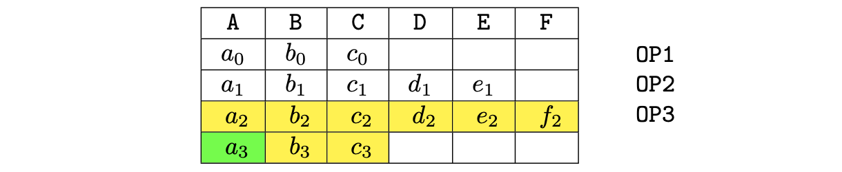
In the above table,

• The yellow cells represent the operands of \(\texttt{Op}\)​3.
• The green cell represents the output of \(\texttt{Op}\)3. i.e., The sum of all the values in the yellow cells.

This time the execution trace has 7 unused cells, which is a big improment compared to the previous 8-column matrix.

Although the columns have reduced, the computation remained the same, and hence the final outcome is also the same.

The input program is still \(\big(\texttt{Op1}, \texttt{Op2}, \texttt{Op3} \big)\). So setting each variable to \(1\) yields the matrix below.

\[ \begin{aligned} \begin{array}{|c|c|c|c|c|c|c|c|}\hline {\texttt{ A }} & {\texttt{ B }} & {\texttt{ C }} & {\texttt{ D }} & {\texttt{ E }} & {\texttt{ F }} \\ \hline \text{1} & \text{1} & \text{1} & \text{} & \text{} & \text{} \\ \hline \text{3} & \text{1} & \text{1} & \text{1} & \text{1} & \text{} \\ \hline \text{7} & \text{1} & \text{1} & \text{1} & \text{1} & \text{1} \\ \hline \text{14} & \text{1} & \text{1} & \text{} & \text{} \\ \hline \end{array} \end{aligned} \]

Example: (Compact execution trace for 2 operations)

Suppose now that the computation involves only two operations; \(\texttt{Op1}\) and \(\texttt{Op}2\).

Let’s examine how to optimize the proving system when the executor’s input program is:

\[ \big( \texttt{Op1}, \texttt{Op}2 \big) \]

Using a 6-column matrix yields the following execution matrix:

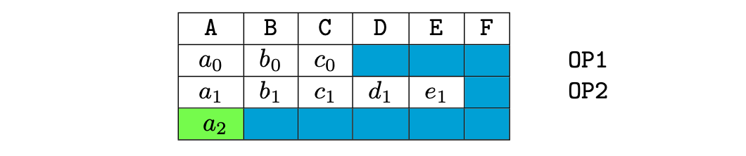
The blue cells, in the above table, represent the unused cells. These are \(9\) in number, constituting exactly 50% of all the cells of the matrix. Such an under utilization of the matrix space is dissatisfactory.

Optimization strategy

An optimal usage of the matrix space can be attained via a strategy similar to the one used in the previous example.

That is, placing the last two operands of \(\texttt{Op}2\) in the last row of the execution matrix. And thus reduce the number of columns from 6 to 3.

\(\texttt{Op}2\) is therefore redefined as follows:

\[ \texttt{OP2}:\ c' = a + b + c + a' + b' \]

The computation’s final outcome is in this case placed in column \(\texttt{C}\), as shown inthe table below.

This revised layout ensures that no cell remains unused, reaching the maximum utilization of the matrix space.

In conclusion, we note that the number of unused cells strongly depends on the executed instructions and the number of columns of the execution matrix.