Intro Generic Sm

In this document is an introduction of the basic components of a generic state machine.

Unlike the mFibonacci state machine, which is an implementation of one specific computation, we now describe a generic state machine that can be instantiated with various computations of the user's choice.

The idea here is to create a state machine that behaves like a processor: it has registers and a clock, it receives programs written in zkASM, and it updates its state at each step according to the current instruction.

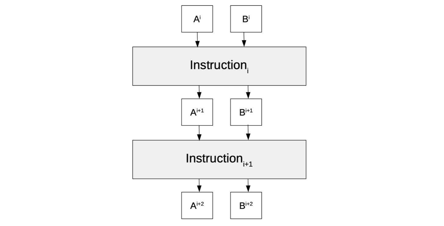
See the figure below for a state machine with registers A and B transitioning from one state to the next based on sequential instructions.

The aim with this document is to explain how the machinery used in the mFibonacci SM; to execute computations, produce proofs of correctness of execution, and verify these proofs; can extend to a generic state machine.

Think of our state machine as being composed of two parts; the part that has to do with generating the execution trace, while the other part is focused on verifying that the executions were correctly executed.

• The former part is more like the 'software' of the state machine, as it is concerned with interpreting program instructions and correctly generating the execution trace. A novel language dubbed the zero-knowledge Assembly (zkASM) language is used in this part.

• But the latter part is more like the 'hardware' as it consists of a set of arithmetic constraints (or their equivalent, polynomial identities) that every correctly generated execution trace must satisfy. Since these arithmetic constraints are transformed into polynomial identities (via an interpolation process), they are described in a novel language called the Polynomial Identity Language (PIL).

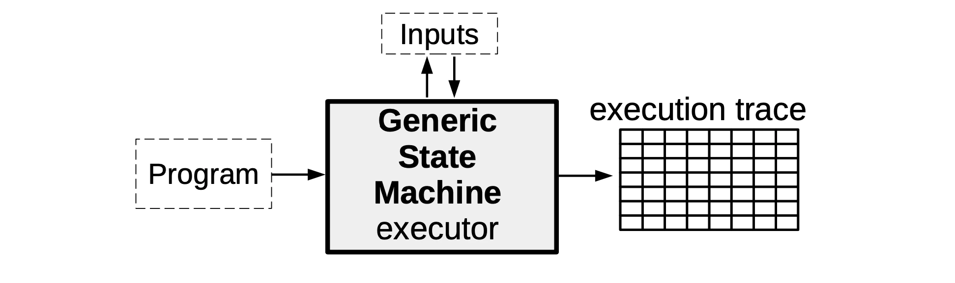
Generic SM executor

As seen with the mFibonacci SM, the SM executor takes certain inputs together with the description of the SM, in order to produce the execution trace specifically corresponding to these inputs.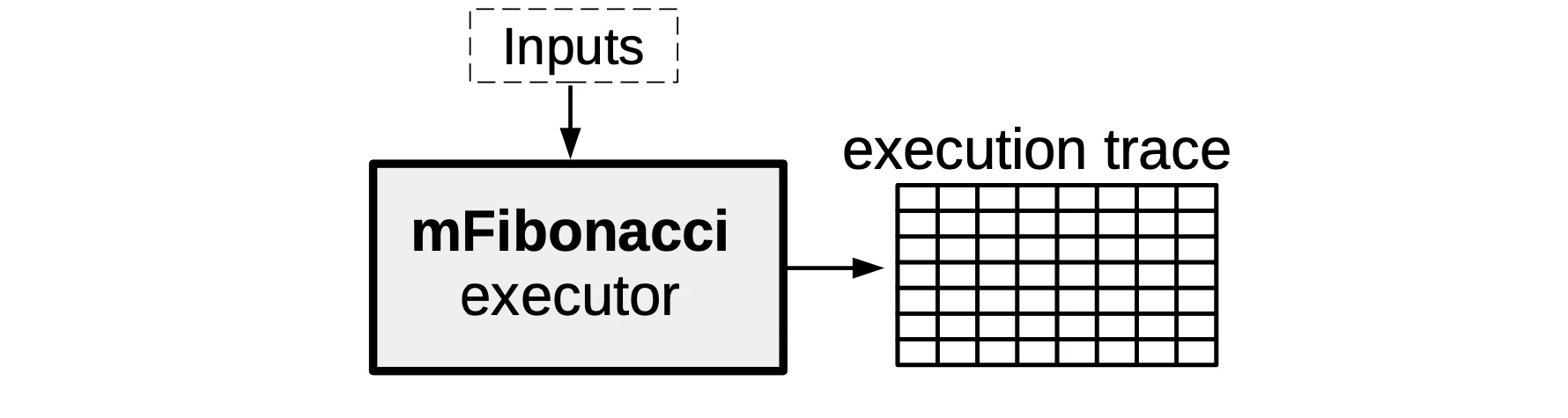

The main difference, in the Generic state machine case, is the inclusion of a program which stipulates computations to be carried out by the SM executor. These computations could range from a simple addition of two register values, or moving the value in register A to register B, to computing some linear combination of several register values.

So then, instead of programming the SM executor ourselves with a specific set of instructions as we did with the mFibonacci SM, the executor of a Generic SM is programmed to read arbitrary instructions encapsulated in some program (depending on the capacity of the SM or the SM's context of application). As mentioned above, each of these programs is initially written, not in a language like Javascript, but in the zkASM language.

State machine instructions

We continue with the model shown in Figure 1: a state machine with two registers (A and B) executing computations as specified by a program.

Here is an example of a program containing four instructions, expressed in the zkASM language,

${getAFreeInput()} => A
3 => B
:ADD
:END

Suppose the state machine starts with the initial state (A, B) = (0, 0). The SM executor sequentially executes each instruction as follows,

• Firstly, ${getAFreeInput()} => A requests a free input value and places it into register A.
• Secondly, 3 => B places the constant value 3 into register B.
• Thirdly, :ADD computes A + B and stores the result into A.
• Lastly, :END resets A and B to their initial values in the next state to achieve cyclic behaviour.

Execution trace

In addition to carrying out computations as per instructions in programs, the executor must also generate the trace of all state transitions, called the execution trace.

Consider, as an example, the execution trace the executor produces for the above program of four instructions. Suppose the free input value used is 7. The generated execution trace can be depicted in tabular form as shown below.

This execution trace utilises a total of six columns. Perhaps the use of the columns corresponding to the two registers A and B, as well as the columns for the constant CONST and the free input FREE, are a bit obvious. But the reason for having the other two columns, A' and B', may not be so apparent.

The reason there are two extra columns, instead of only four, is the need to capture each state transition in full, and per instruction. The column labelled A' therefore denotes the next state of register A, and similarly, B' denotes the next state of register B. This ensures that each row of the execution trace reflects the entire state transition pertaining to each specific instruction.

The execution trace is therefore read row-by-row as follows,

• The first row (per ${getAFreeInput()} => A) gets the free input value 7 and sets the next A value to 7.
• The second row (per 3 => B) moves the constant value 3 into register B as its next value, and A remains at 7 as expected.
• The third row (per :ADD) computes the sum of register values in A and B (i.e. 7 + 3 = 10) and moves the output 10 into register A as its next value.
• The last row (per :END) resets registers A and B to zeros (their initial values) as their next values.

Note that, for this specific program, a change in the free input from 7 to another number would obviously yield a different execution trace, yet without violating the first instruction.